By the end of this blog post, you will have a better understanding of APIs and their benefits for researchers, and moreover, you will have built your own API wrapper, and possibly, even your own API endpoints. Most importantly, the in-depth walkthrough will hopefully help you identify APIs in the wild. You will realize that APIs are used everywhere, from the KOF Data API1, to Art Museums and COVID-19 case rates.
Let’s go back to the initial of an economic index. How would we approach gathering data to build our economic index?
The Naive Way of collecting data would be to google for relevant data. Like in most countries, in Switzerland, the Federal Statistical Office (FSO) is a good source for information such as the GDP - the most common representation in macroeconomics for a country’s economic activity.
By clicking on the search result of the FSO website, we could find their Economic Data Portal.

Then, after searching for our desired time series, we would find different variations of GDP data.
After downloading the dataset from the FSO, we can open and inspect it. The data is typically downloaded in Microsoft Excel file format and represented in wide format (meaning values are horizontally oriented) because it is more humanly readable than other more compact representations.
When programming though, we often prefer the so-called long format (values vertically oriented) because it makes plotting and cleaning of data easier. Particularly time series data is represented in this way2.
So, once downloaded, we have to transform the data from wide to long format, so it is more handleable for us.
library(readxl)
library(magrittr)
library(tidyr)

data <- read_xlsx("je-d-04.02.01.03.xlsx")

# subset only the rows 3 (= year) and 9 (= gdp)
gdp <- data[9,]
names(gdp) <- data[3,]

# pivot data longer (from excel wide format to data frame long format)
gdp_long <- gdp %>%
  pivot_longer(
    cols = everything(),
    names_to = "Year",
    values_to = "GDP"
  )

# remove old headers
gdp_long <- gdp_long[-c(1:2),]

# check structure
# str(gdp_long)

# convert to gdp numeric and year to year
gdp_long$GDP <- as.numeric(gdp_long$GDP)
gdp_long$Year <- as.integer(gdp_long$Year)

head(gdp_long, n=10)
We read in our data, then select the rows which we need, which is the aggregated GDP, and the date. Then we pivot our data (which transforms the data from horizontally oriented to vertically oriented), and remove old headers. Finally, we check that our data is correctly represented in the desired format:
::: cell
::: {.cell-output .cell-output-stdout}
# A tibble: 10 × 2
Year GDP
By now, we have successfully searched for, imported and cleaned our first time series dataset for our Economic Index.
It was quite a long and intensive process, wasn’t it? We had to look for the correct data, download, and then clean it. Given that we have approximately 299 time series to go to build our index, this approach could become quite unsustainable quickly --- especially if we want to repeat this process in the future to update our index.
Moreover, while GDP is such a common dataset and hence is readily available and published in a well known format, this might not be the case for more niche time series. Finding, importing and cleaning other time series could become a lot more difficult..
Hence, let’s introduce a different method for extracting data from a public source that is more repeatable, and reproducible (we want to do it using code).
The reason why APIs are preferred as data source over the Naive Way is that when using APIs everything is standardized, thanks to protocols.
API stands for Application Programming Interface, and essentially standardizes the way in which your computer communicates with another computer. Protocols are just explicit set of rules which need to be followed. Most APIs use something called HTTP - which dictates how all data transfer happens over the web. You might have already seen HTTP in your browser (e.g. http://url…) this is because your browser on your computer and the webserver also communicate via HTTP.
But just communicating via http:// in our browser is not enough. This approach is still not reproducible, since we need to input the urls every time we want to get our data. We want to find a solution that is reproducible and uses code. In other words, we want our R code to communicate with the server - so we use APIs.
There are two important things I want you to know about HTTP:


Now that we focus on APIs that use the HTTP protocol, let’s put it all together to explain what an API looks like.
The request (which is how we communicate to the server what we want it to do) consists of:

/users/{userID} or/users?ID=userID (& can also be used
to separate multiple body params)
Once a request is sent to the server, it gives back a response:

Let’s use what we’ve learnt to look at an example:

The Museum of Modern Art has an API which can be used to determine what kind of artworks they have, based on certain keywords in the artworks title.
Example URL: https://collectionapi.metmuseum.org/public/collection/v1/search?q=bread
This is a GET request to the Met Museum Collection API. It consists of:
The API returns JSON containing the total number of matching objects and an array of objectIDs for items that match the keyword. Try pasting the URL into your browser and replace “bread” with any other keyword to see different results.
I encourage you to try out GET API call yourself, by putting in the URL of the Example into your browser and inputting your own search word. Since HTTP is used on the web, we can perform the GET request via our browser as well.
The most frequent way we as developers encounter APIs is through so called API wrappers. You can think of them like simple programs that are give an entrypoint through a function in your favorite programming language that takes input parameters and puts together the right API Url and request based on that input. In other words, they wrap the API.
API wrappers usually allow you to do complex API calls in an easier environment and are tailored to your programming language, so they are usually the most convenient way for us to use an API.

Here is a visual example of how you might encounter an API wrapper. Notice how the functionality stays the same, we can perform the same tasks, but we see and interact with less complexity. This is something we call information hiding.
There are many API wrappers in R that you can use for your future analyses, to name a few:
Let’s go back to our example of getting data from the Swiss Federal Statistical Office (FSO). Since we have already imported and cleaned our GDP data, we want to move on to the next relevant time series. One other factor that could be a good predictor for economic activity in Switzerland is energy consumption over time.
Luckily, we can use the FSO’ API wrapper, which is the BFS’ R Package to get our energy data.
# devtools::install_github("lgnbhl/BFS")
library(BFS)

# to inspect functions, use ?function, e.g.
?bfs_get_catalog_data

catalog <- bfs_get_catalog_data(language = "en", title = "energy")
dataset_nr <- catalog$number_bfs[1]
energy_df <- bfs_get_data(dataset_nr, lang = "en")

# filter only total energy accounts
total_energy <- subset(
  energy_df,
  # filter for totals for each of the columns
  `Economy and households` == "Economy and households - Total" &
  `Energy product` == "Energy product - Total",
  # select only the two relevant columns
  select = c(Year, `Energy accounts of economy and households`)
)

names(total_energy)[2] <- "Amount"

# View(total_energy)
head(total_energy, n=10)
Let’s go through the code line-by-line:
First we install and load the package, then we can inspect the functions
we will use, such as bfs_get_catalog_data to see that we can use this
function to determine what kind of data BFS publishes, based on
keywords.
::: cell
::: {.cell-output .cell-output-stdout}
# A tibble: 1 × 6
title language number_bfs number_asset publication_date url_px
We search for energy datasets, save the respective ID of the dataset,
and then GET the data, using the bfs_get_data function.
After line 9, we are already done with the API usage for this example. The rest is just filtering the dataset to get only the columns of interest (total Energy Product across all Economy and Households)
When inspecting the data, it looks like this:
| Year | Amount |
|---|---|
| 2006 | 1157170 |
| 2007 | 1126804 |
| 2008 | 1158734 |
| 2009 | 1136915 |
In theory, we could be done with this example - using API wrappers instead of manually looking for data on the web makes it easier for us to scale our example - meaning we can easily fetch our 300 time series with little extra effort.
Still, to get a deeper understanding of how APIs work, we could also
take a look at how API Wrappers work under the hood. Luckily for us, R
packages like FSO are open source (like the R programming language) so
we can see how a function such as bfs_get_data is written. We can go
to the Package author’s github page, and find the
function
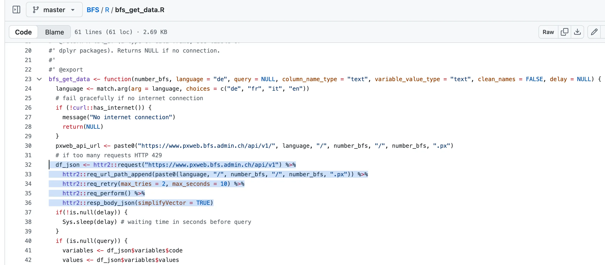
This might look a bit complex, so let’s break it down by looking at the essential code:
bfs_get_data <- function(number_bfs, language = "de", query = NULL, column_name_type = "text", variable_value_type = "text", clean_names = FALSE, delay = NULL) {
  # base url
  df_json <- httr2::request("https://www.pxweb.bfs.admin.ch/api/v1") %>%
    # add path params
    httr2::req_url_path_append(paste0(language, "/", number_bfs, "/", number_bfs, ".px")) %>%
    httr2::req_retry(max_tries = 2, max_seconds = 10) %>%
    # executre request
    httr2::req_perform() %>%
    # transform response to json
    httr2::resp_body_json(simplifyVector = TRUE)
<!-- TODO: add explanation about pxweb -->In essence, the function uses the existing API to build a request, then perform it, and save the response body.
Here, we build the request with the base URL, then append this URL with our path parameters which are the dataset ID and the language, and then perform the request and specify that the response body (which contains the data) should be in JSON.
Important to mention here, is that these above functions are used to fetch the general structure of the data, i.e. the units, and different data categories. This information is then being used to fetch the actual data via the px-web API which is a way of distributing data that statistical offices like to use. In principle, we could also use the functions presented above to get the data, and other API wrappers in R that you can find do so.
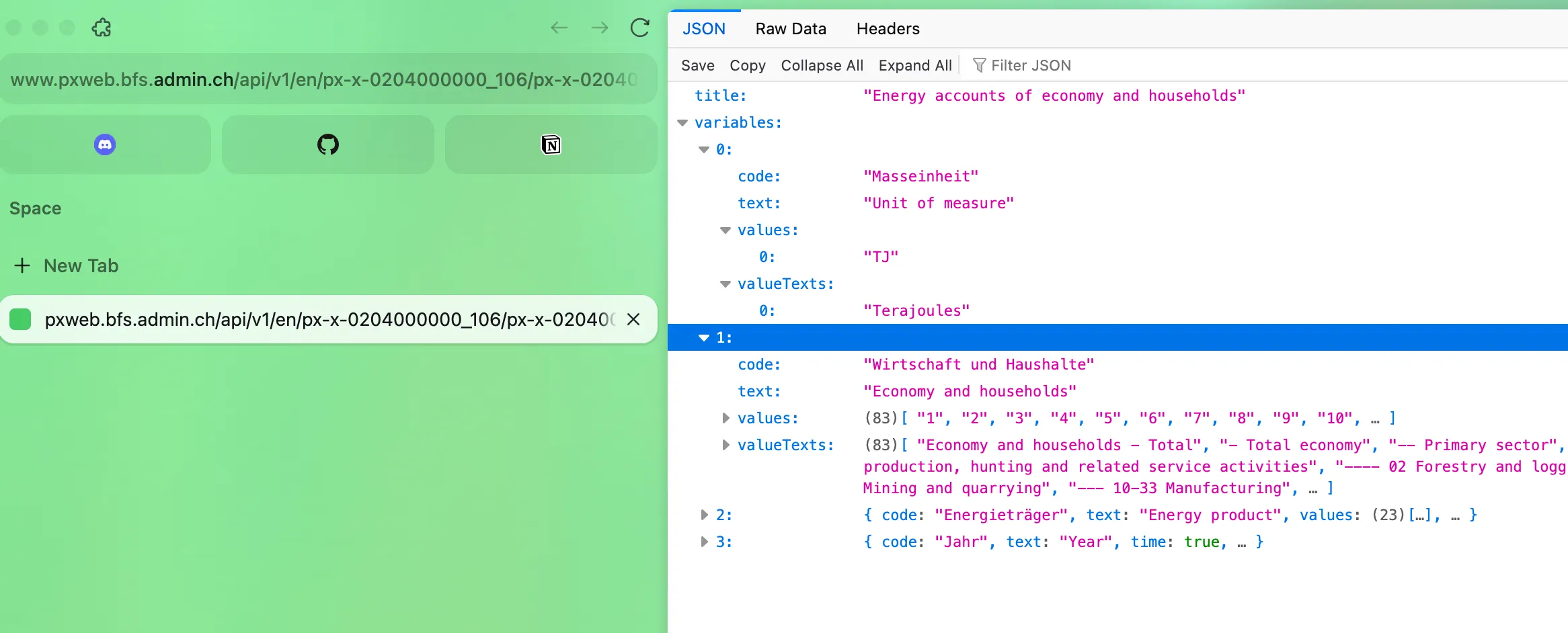
We can also try running the final URL which we create with the above functions (up to line 5) in our browser3, as we did before, to see what the structure of our data looks like:
By now you might have gathered an idea about why APIs are important and it’s good practice to use them in research.
Here are some additional benefits:
Now that APIs have been thoroughly introduced and their importance is clearer, try to build your own API wrapper.
Most commonly used APIs already have pre-built API wrappers, but it could be that they are not available in your programming language of choice, or are not maintained, or they don’t exist at all. In that case, knowing how to go about building your own API wrapper could be very useful.
In R, the most commonly used package to work with the HTTP protocol is the httr2 package - on their website, you can find the documentation to get started with using httr2. A short cheatsheet summarizes the essential functions:
| Category | Function | Description |
|---|---|---|
| Request | request() | Creates a new HTTP request object that defines the endpoint and method (e.g., GET, POST). |
| Request | req_perform() | Sends the built request to the server and returns the response object. |
| Response | resp_body_json() | Parses the response body as JSON and returns it as an R list. |
| Response | resp_status() | Retrieves the HTTP status from the response object. |
Let’s take stock of the datasets that we’ve gathered so far: we have Swoss GDP and energy consumption. Now, let’s say we want to look at how the COVID pandemic has affected the Swiss Economy. To understand this better, we would need to look at COVID case and vaccination rates.
Luckily, the disease.sh docs provides not only an open API for disease-related statistics, but also nice API documentation. We can look at various APIs and try out their endpoints! Try it out!
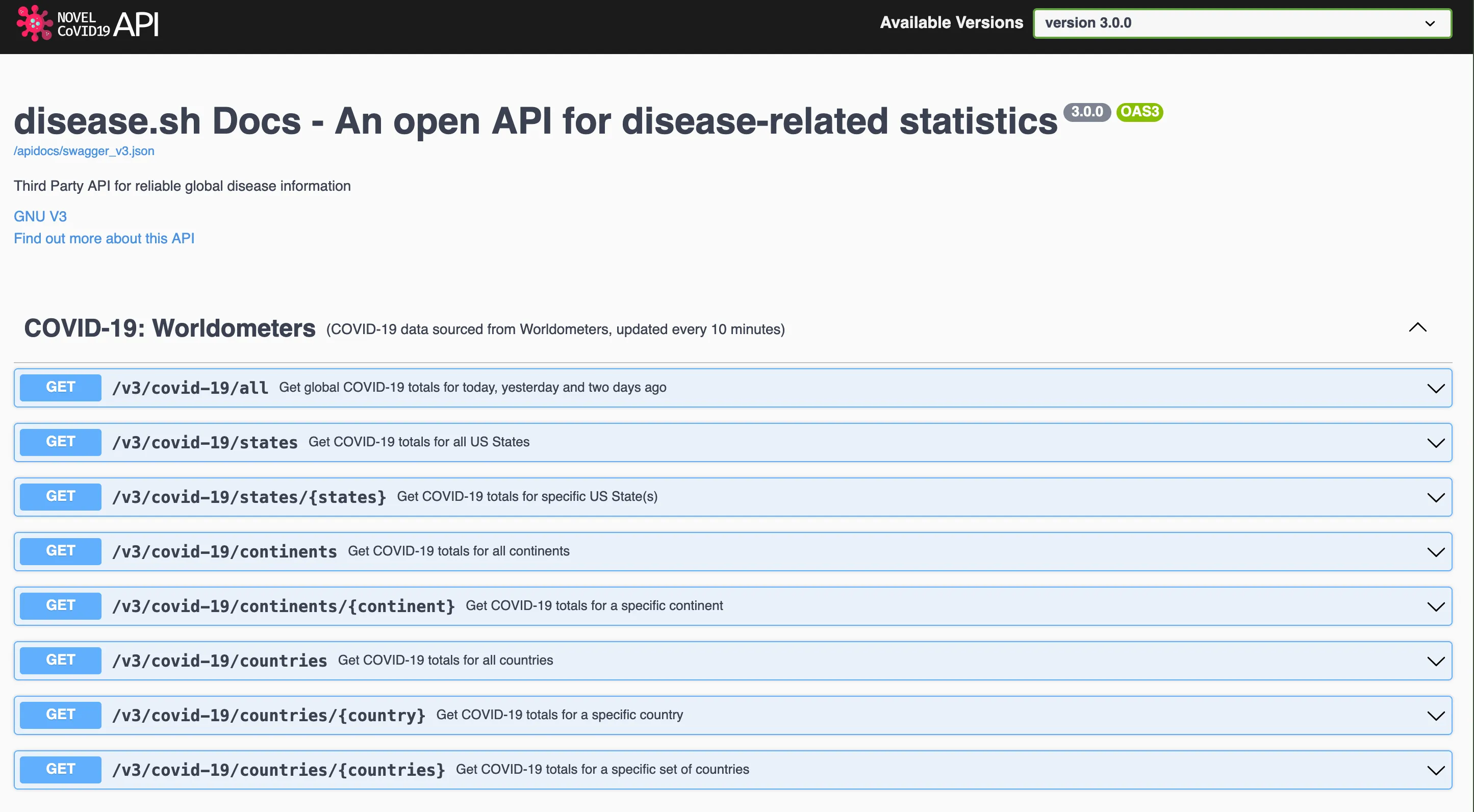
Here we can see various COVID-19 APIs, such as from Worldometer or Johns Hopkins University.
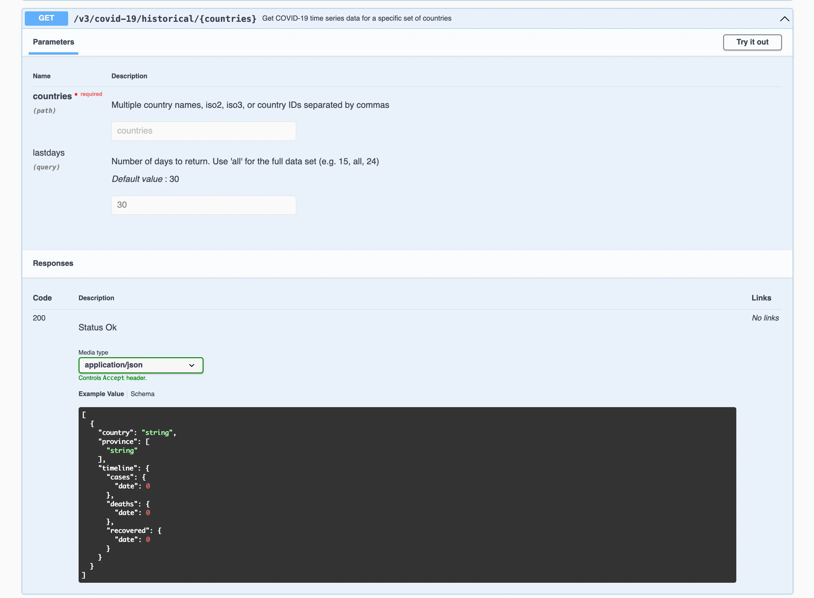
Selecting one endpoint to try out, we can identify the historical case counts of certain countries.
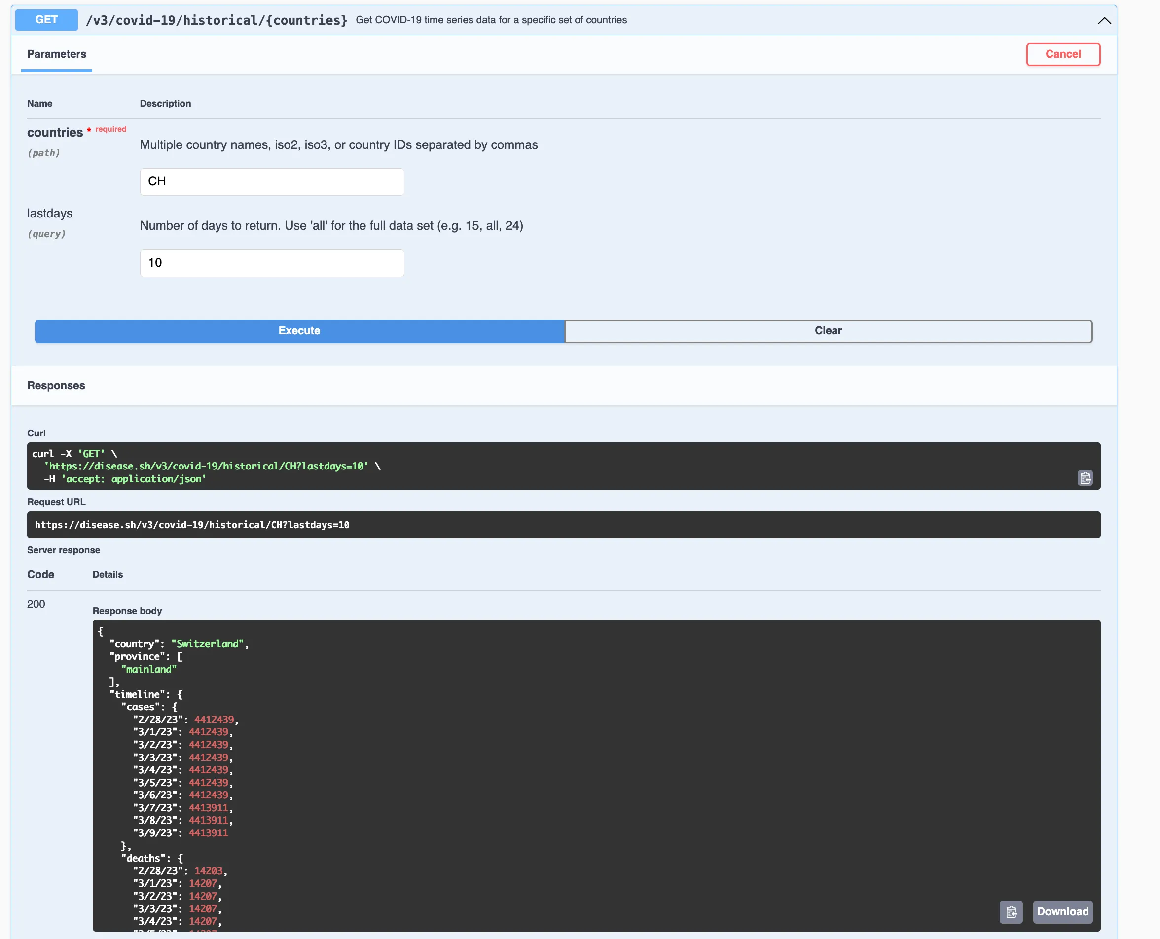
When trying out the endpoint, we can even get the data as responses, and see all of the components of a real API call.
Let’s try to turn this example into an actual function:
library(httr2)

get_case_counts <- function(country = "CH", period = c(30,365, "all")){
  # "https://disease.sh/v3/covid-19/historical/CH?lastdays=30"
  # this way is error prone, try to match.args to check if the inputs are correct
  base_url <- "https://disease.sh/v3/covid-19/historical"
  final_url <- paste0(base_url, "/", country, "?lastdays=", period)

  # perform API call with httr2
  req <- request(final_url)
  resp <- req_perform(req)

  # if request is not successful
  if (resp_status(resp) != 200){
    message("The request was not successful")
  }
  else{
    return(resp_body_json(resp))
  }
}

get_case_counts("CH", 1)
When running the last line get_case_counts("CH", 1) we get the
following output
    $country
    [1] "Switzerland"

    $province
    $province[[1]]
    [1] "mainland"


    $timeline
    $timeline$cases
    $timeline$cases$`3/9/23`
    [1] 4413911


    $timeline$deaths
    $timeline$deaths$`3/9/23`
    [1] 14210


    $timeline$recovered
    $timeline$recovered$`3/9/23`
    [1] 0
Here it’s important to note that the Johns Hopkins University apparently stopped releasing this data after 3.9.2023 and it does seem a bit implausible that there are 0 recoveries on that day - alas!
Use the same documentation as above (disease.sh docs) to get the historical vaccination doses delivered for a specific country. Try out the desired endpoint using the documentation, before writing your own function. Feel free to use this function as a template:
library(httr2)

get_country_vaccine_counts <- function(country = "CH", period = c(30,365, "all")){

  base_url <- "..."
  final_url <- "..."

  # perform  API call with httr2
  req <- "..."(final_url)
  resp <- "..."(req)

  # if request is not successful
  if (resp_status(resp) != 200){
    message("The request was not successful")
  }
  else{
    return(resp_body_json(resp))
  }
}
Try out your built function! What does it return4 ? Congratulations on adding one more dataset to your collection for your economic indicator.
In case this is still not enough for you, and you not only want to know how to use and build API wrappers, but you also want to build your own (web) API, I’ve got another exercise for you.
In R, with the plumber R package supports you to create your own API. By following this exercise, you will get an even deeper understanding of what APIs do, Plumber is a lightweight R package that turns R functions into web APIs.
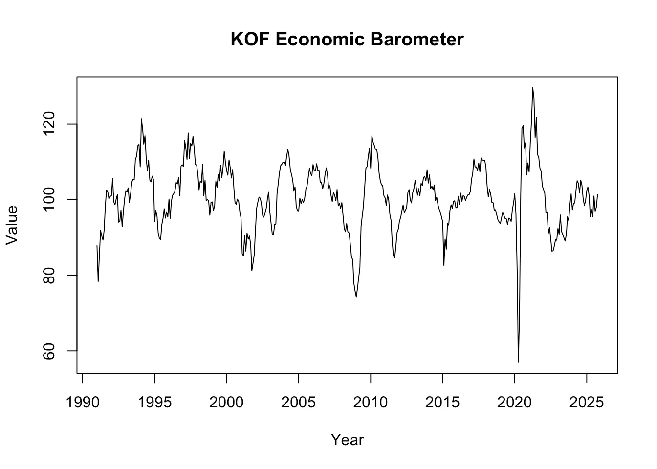
For example you could use the plumber package to replicate the KOF API, which provides users with the ability to get different public time series data which the Swiss Economic Institute (KOF-ETH) produces and provides.
Think of building this API and its endpoints as a different service your API restaurant offers. Or, think of it like the layers of an onion: start simple, then add layers of functionality as needed. Begin with the outermost, easiest layer:
GET HTTP request/datalibrary(plumber)
#* Return entire KOF Barometer time series
#* @get /data
function() {
# the partition_ts function will be explained below!
partition_ts(data$kofbarometer)
}When you run your API, you get an interactive documentation interface (called Swagger) that looks like this:
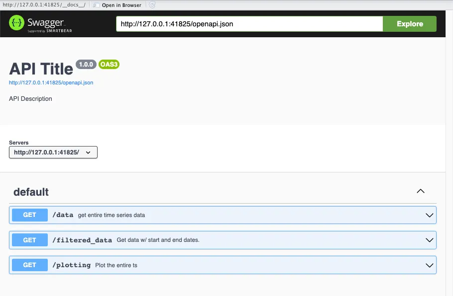
Important to note here, is that you can see 3 different endpoints here
(/data, /filtered_data and /plotting because those are the 3
endpoints we will create throughout this example, for now, just focus on
the endpoint we just created: /data)
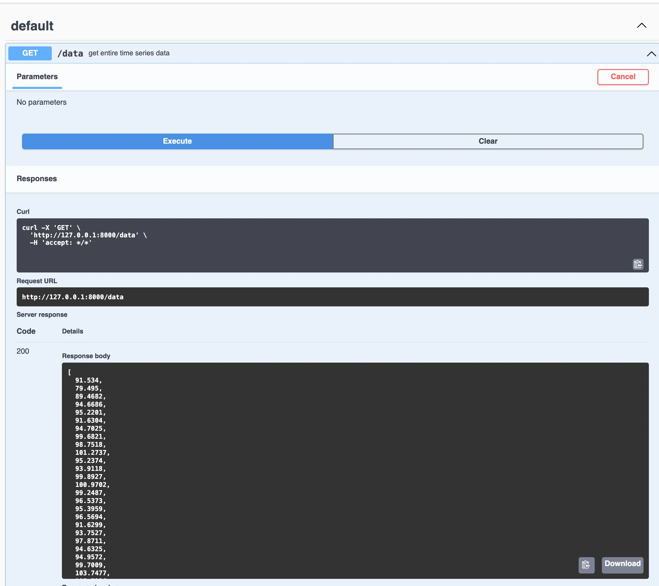
Since we just created the /data endpoint, see code snippet above, we
will try it out and see the Response Body, which contains the entire
Konjunkturbarometer time series.
/filtered_data which/data?start=2020&end=2024 (Hint: these are the query
parameters we introduced before)For this, we first need to create a function partition_ts which takes
the parameters the API users pass to the endpoint, i.e. a start and end
date. We then partition the time series according to those parameters.
#* @param ts time series object
#* @param start date at which ts should start - can be years only, or c(year, month)
#* @param end date at which ts should end - can be years only, or c(year, month)

partition_ts <- function(ts, start = NULL, end = NULL) {
  if (inherits(ts, "ts")) {
    # setting start and end date if unset
    if (is.null(end)) {
      end <- time(ts)[length(ts)]
    }
    if (is.null(start)) {
      start <- time(ts)[1]
    }
    # filter ts based on start & end dates
    ts <- window(ts, start = start, end = end)
  } else {
    warning("Input is not a ts object")
    return(NULL)
  }
  return(ts)
}
We use the partition_ts function to create our new endpoint function
#* Return KOF Barometer data with custom date range
#* @param start the start year to filter by
#* @param end the end year to filter by
#* @get /filtered_data
function(start = NULL, end = NULL) {
  if (!is.null(start)) {
    start <- as.numeric(start)
  }
  if (!is.null(end)) {
    end <- as.numeric(end)
  }

  partition_ts(
    data$kofbarometer,
    start = start,
    end = end
  )
}
Let’s create our own API that shares KOF Barometer data. We’ll build endpoints where users can:
/data?start=2020&end=2024/plotLet’s test the /filtered_data endpoint by requesting KOF Barometer
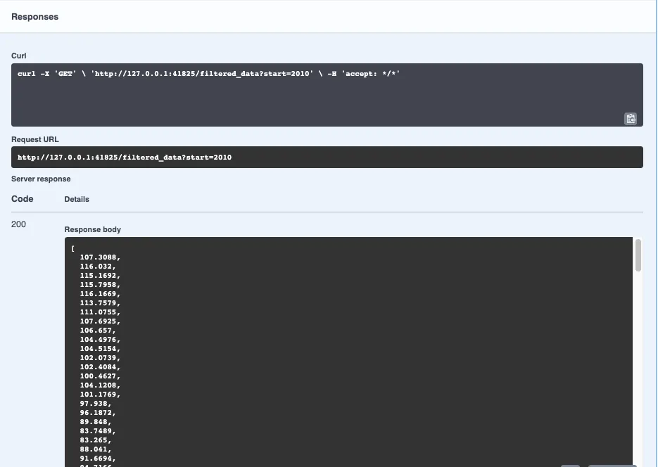
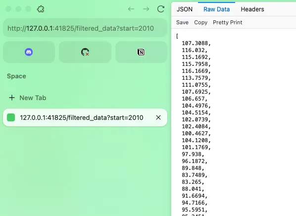
data from 2010 onwards:
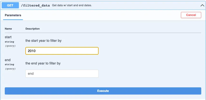
Hit “Execute” and voila---the Server response shows the exact data requested:
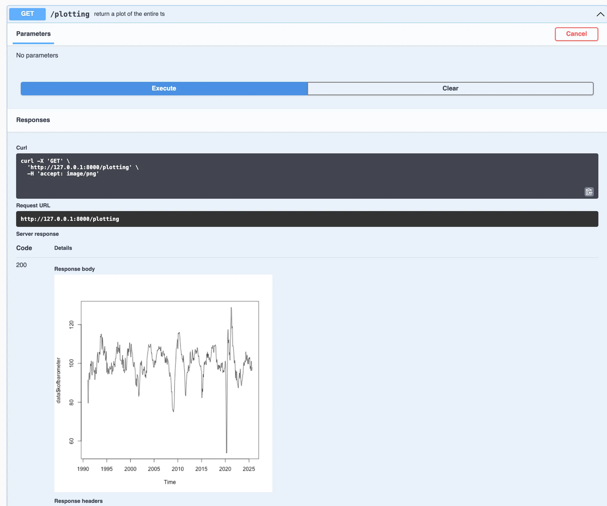
/plotting endpointGET request, we return ready-made charts:#* Return KOF Barometer chart as PNG
#* @serializer png
#* @get /plotting
function() {
plot(data$kofbarometer)
}
Important to Note: The images you see above is the API Documentation which is automatically generated when using the plumber R package. Swagger is your API’s user-friendly interface, but behind the scenes, your API users will interact with your API through HTTP requests, as already shown above. In this example, a Get Request can be executed in the browser like this:
If you want to test out how to use the plumber R package to create your own API, incl. the API documentation , then I encourage you to do so. However, for this, consult the plumber documentation and make sure to do this:
Testing Your API Locally
Save all three functions in a file called
plumber.Rin the base of your working directory, then launch your API:# Launch your API on port 8000 pr("plumber.R") %>% pr_run(port=8000)
Congratulations! You’ve just built your own API!
I hope you were able to learn something through this blog post, whether that is how APIs and APIs wrapper work and look like, or even how to build your own API (wrapper). Please find additional information on the HSG Data Handling Lecture on their GitHub repository5. In case you have any questions, feel free to contact me at heim [ at ] kof.ethz.ch.
https://kof.ethz.ch/en/forecasts-and-indicators/indicators/kof-economic-barometer.html ↩
https://www.dontusethiscode.com/blog/2024-11-20_pandas_reshaping.html ↩
Try executing the Get Request yourself in your browser: https://www.pxweb.bfs.admin.ch/api/v1/en/px-x-0204000000_106/px-x-0204000000_106.px ↩
If you want to take a look at a sample solution of this task, check out: https://minnaheim.github.io/dh_guest_lecture_2025/presentation.html#/get-vaccine-rates ↩
HSG Data Handling Lecture repository: https://github.com/ASallin/datahandling-lecture ↩