6 Case Studies
While the rest of the book provided more of a big picture type of insight, this section is all about application minded examples that feature code to reproduce.
6.1 Consuming APIs
An Application Programming Interface (API) is nothing else but an interface to facilitate machine to machine communication. An interface can be anything, any protocol or pre-defined process. But of course there are standard and not-so-standard ways to communicate. Plus some matter-of-taste type of decisions. But security and standard compliance are none of the latter. There are standards such as the popular, URL based REST that make developers’ lives a lot easier – regardless of the language they prefer.
Many services such as Google Cloud, AWS, your university library, your favorite social media platform or your local metro operator provide an API. Often either the platform itself or the community provide what’s called an API wrapper:
A simple program wraps the process of using the interface though dynamic URLs into a parameterized function. Because the hard work is done serverside by the API backend, building API wrappers is fairly easy and if you’re lucky wrappers for your favorite languages exit already. If that is the case end users can simply use functions like get_dataset(dataset_id) to download data programatically.
6.1.1 Example 1: The {kofdata} R package
The KOF Swiss Economic Institute at ETH Zurich provides such a wrapper in an R package. The underlying API allows to access the KOF time series archive database and obtain data and meta information alike. The below code snippet gets data from the API and uses another KOF built library ({tstools}) to visualize the returned time series.
library(kofdata)
# just for viz
library(tstools)
tsl <- get_time_series("ch.kof.barometer")
tsplot(tsl)
6.1.2 Example 2: The {OECD} R package
Also large organizations like the Organization for Economic Co-operation and development (OECD) provide API wrappers to facilitate data consumption.
6.1.3 Build Your Own API Wrapper
Here’s an example of a very simple API wrapper that makes use of the Metropolitan Museum of Modern Art’s API to obtain identifiers of pictures based on a simple search.
# Visit this example query
# https://collectionapi.metmuseum.org/public/collection/v1/search?q=umbrella
# returns a json containing quite a few ids of pictures that were tagged 'umbrella'

#' Search MET
#'
#' This function searches the MET's archive for keywords and
#' returns object ids of search hits. It is a simple wrapper
#' around the MET's Application Programming interface (API).
#' The function is designed to work with other API wrappers
#' and use object ids as an input.
#' @param character search term
#' @return list containing the totoal number of objects found
#' and a vector of object ids.
#'
# Note these declaration are not relevant when code is not
# part of a package, hence you need to call library(jsonlite)
# in order to make this function work if you are not building
# a package.
#' @examples
#' search_met("umbrella")
#' @importFrom jsonlite formJSON
#' @export
search_met <- function(keyword){
  # note how URLencode improves this function
  # because spaces are common in searches
  # but are not allowed in URLs
  url <- sprintf("https://collectionapi.metmuseum.org/public/collection/v1/search?q=%s", URLencode(keyword))
  fromJSON(url)
}
You can use these ids with another endpoint in order to receive the pictures themselves.
download_met_images_by_id <- function(ids,
                                      download = "primaryImage") {
  # Obtain meta description objects from MET API
  obj_list <- lapply(ids, function(x) {
    req <- download.file(sprintf("https://collectionapi.metmuseum.org/public/collection/v1/objects/%d",
                   x),destfile = "temp.json")
    fromJSON("temp.json")
  })

  # Extract the list elements that contains
  # img URLs in order to pass it to the download function
  img_urls <- lapply(obj_list, "[[", download)
  # Note the implicit return, no return statement needed
  # last un-assigned statement is returned from the function
  lapply(seq_along(img_urls), function(x) {
    download.file(img_urls[[x]],
                  destfile = sprintf("data/image_%d.jpg", x)
    )
  })
}


# Step 4: Use the Wrapper
umbrella_ids <- search_met("umbrella")
umbrella_ids
download_met_images_by_id(umbrella_ids$objectIDs[2:4])
6.2 Create Your Own API
Being able to expose data is a go-to skill in order to make research reproducible and credible. Especially when data get complex and require thorough description in order to remain reproducible for others, a programmtic, machine readable approach is the way to go.
6.2.1 GitHub to Serve Static Files
Exposing your data through an API is not something you would need a software engineer or an own server infrastructure for. Simply hosting a bunch of .csv spreadsheet alongside a good description (in separate files!!) on, e.g., GitHub for free can be an easy highly available solution to serve static files.
The KOF High Frequency Economic Monitoring dashboard simply shares standardized .csv (data) and .json (description) files based on a Github.
INSERT SCREENSHOT OF GITHUB HERE
To make it look at little niftier, the dashboard uses a quasar frontend to guide the human user, but it would not be necessary to have such a framework.
INSERT SCREENSHOT OF KOFDATA HERE
6.2.2 Simple Dynamic APIs
Even going past serving static files, does not require much software development expertise. Thanks to frameworks such as express.js or the {plumbr} it easy to create an API that turns a URL into a server side action and returns a result.
Assume you’ve installed node.js already, you can set up a simple API on your local computer just like this.
# run initialization in a dedicated folder
mkdir api
cd api
npm init
just sleep walk through the interactive dialog accepting all defaults. Once done, add install express using the npm package manager.
npm install express --save6.3 A Minimal Webscraper: Extracting Publication Dates
Even though KOF Swiss Economic Institute offers a REST API to consume publicly available data, publication dates are unfortunately not available through in API just yet. Hence, in order to automate data consumption based on varying publication dates, we need to extract upcoming publication dates of the Barometer from KOF’s media release calendar. Fortunately all future releases are presented online an easy-to-scrape table. So here’s the plan:
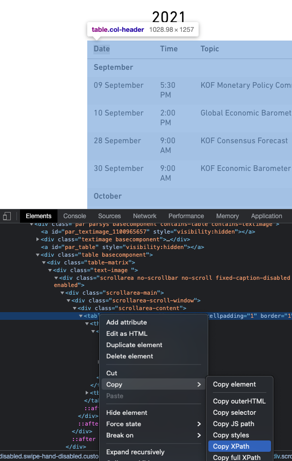
Use Google Chrome’s inspect element developer feature to find the X-Path (location in the Document Object Model) of the table.
Read the web page into R using
rvest.Copy the X-Path string to R to turn the table into a data.frame
use a regular expression to filter the description for what we need.
Let’s take a look at our starting point, the media releases sub page, first.
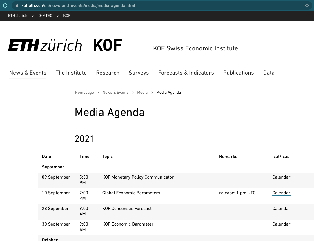
The website looks fairly simple and the jackpot is not hard, presented in a table right in front of us. Can’t you smell the data.frame already?
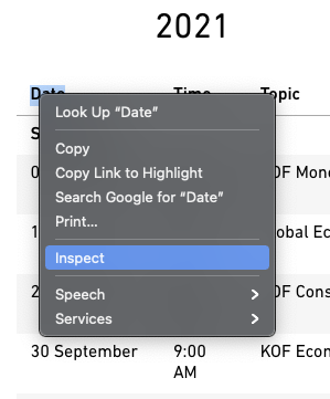
Right click the table to see a Chrome context window pop up. Select inspect.
Hover over the blue line in the source code at the bottom. Make sure the selected line marks the table. Right click again, select copy -> copy X-Path.
On to R!
library(rvest)
# URL of the media release subsite
url <- "https://kof.ethz.ch/news-und-veranstaltungen/medien/medienagenda.html"

# Extract the DOM object from the path we've previously detected using
# Chrome's inspect feature
table_list <- url %>%
  read_html() %>%
  html_nodes(xpath = '//*[@id="contentMain"]/div[2]/div/div[3]/div/div/div/div/div/div/table') %>%
  # turn the HTML table into an R data.frame
  html_table()

# because the above result may potentially contain multiple tables, we just use
# the first table. We know from visual inspection of the site that this is the
# right table.
agenda_table <- table_list[[1]]

# extract KOF barometer lines
pub_date <- agenda_table[grep("barometer",agenda_table$X3),]
pub_date
## # A tibble: 2 × 5
## X1 X2 X3 X4 X5
## <chr> <chr> <chr> <chr> <chr>
## 1 30. Nov. 9:00 KOF Konjunkturbarometer "" Kalendereint…
## 2 30. Dez. 9:00 KOF Konjunkturbarometer "" Kalendereint…Yay! We got everything we wanted. Ready to process.
6.4 Automate Script Execution: A GitHub Actions Example
6.5 Choropleth Map: Link Data to a geojson Map File
Data visualization is a big reason for researchers and data analysts to look into programming languages. Programming languages do not only provide unparalleled flexibility, they also make data visualization reproducible and allow to place charts in different contexts, e.g., websites, printed outlets or social media.
One of the more popular type of plots that can be created smoothly using a programing language is the so called choropleth. A choropleth maps values of a variable that is available by region to a given continuous color palette on a map. Let’s break down the ingredients of the below map of Switzerland.
First, we need a definition of a country’s shape. Those definitions come in various format from traditional shape files to web friendly geoJSON. Edzer Pebesma’s useR! 2021 keynote has a more thorough insight.
Second, we need some data.frame that simply connects values to regions. In this case we use regions defined by the Swiss Federal Statistical Office (FSO). Because our charting library makes use of the geoJSON convention to call the region label ‘name’ we need to call the column that holds the region names ‘name’ as well. That way we can safely use defaults when plotting. Ah, and note that the values are absolutely bogus that came to my mind while writing this (so please do not mull over how these values were picked).
d <- data.frame(
  name = c("Zürich",
           "Ticino",
           "Zentralschweiz",
           "Nordwestschweiz",
           "Espace Mittelland",
           "Région lémanique",
           "Ostschweiz"),
  values = c(50,10,100,50,23,100,120)
)
Last but not least where calling our charting function from the echarts4r package. echarts4r is an R wrapper for the feature rich Apache Echarts Javascript plotting library. The example uses the base R pipes (available from 4+ on, former versions needed to use pipes via extension packages.). Pipes take the result of one previous line and feed it as input into the next line. So the data.frame d is linked to a charts instance and the name column is used as the link. Then a map is registered as CH and previously read json content is used to describe the shape.
d |>
  e_charts(name) |>
  e_map_register("CH", json_ch) |>
  e_map(serie = values, map = "CH") |>
  e_visual_map(values,
               inRange = list(color = viridis(3)))
Also note the use of the viridis functions which returns 3 values from the famous, colorblind friendly viridis color palette.
viridis(3)## [1] "#440154FF" "#21908CFF" "#FDE725FF"Here’s the full example:
library(echarts4r)
library(viridisLite)
library(jsonlite)

json_ch <- jsonlite::read_json(
  "https://raw.githubusercontent.com/mbannert/maps/master/ch_bfs_regions.geojson"
)


d <- data.frame(
  name = c("Zürich",
           "Ticino",
           "Zentralschweiz",
           "Nordwestschweiz",
           "Espace Mittelland",
           "Région lémanique",
           "Ostschweiz"),
  values = c(50,10,100,50,23,100,120)
)

d |>
  e_charts(name) |>
  e_map_register("CH", json_ch) |>
  e_map(serie = values, map = "CH") |>
  e_visual_map(values,
               inRange = list(color = viridis(3)))
6.6 Web Applications /w R Shiny
For starters, let me de-mistify {shiny}. There are basically two reasons why so many inside data science and analytics have shiny on their bucket list of things to learn. First, it gives researchers and analysts home court advantage on a webserver. Second, it gives our online appearances a kickstart in the dressing room.
Don’t be surprised though if your web development professional friend outside data science and analytics never heard of it. Compared to web frontend framework juggernauts such as react, angular or vue.js the shiny web application framework for R is rather a niche ecosystem.
Inside the data science and analytics communities, fancy dashboards and the promise of an easy, low hurdle way to create nifty interactive visualizations have made {shiny} app development a sought after skill. Thanks to pioneers, developers and teachers like Dean Attali, John Coene, David Granjon, Colin Fay and Hadley Wickham, the sky seems the limit for R shiny applications nowadays.
This case study does not intend to rewrite {shiny}’s great documentation or blogs and books around it. I’d rather intend to help you get your first app running asap and explain a few basics along the way.
6.6.1 The Web Frontend

Stats & figures put together by academic researchers or business analysts are not used to spend a lot of time in front of the mirror. (Often for the same reason as their creators: perceived opportunity costs.)
Shiny bundles years worth of lime light experience and online catwalk professionalism into an R package. Doing so allows us to use all this design expertise through an R interface abstracting away the need to dig deep into web programming and frontend design (you know the HTML/CSS/Javascript).
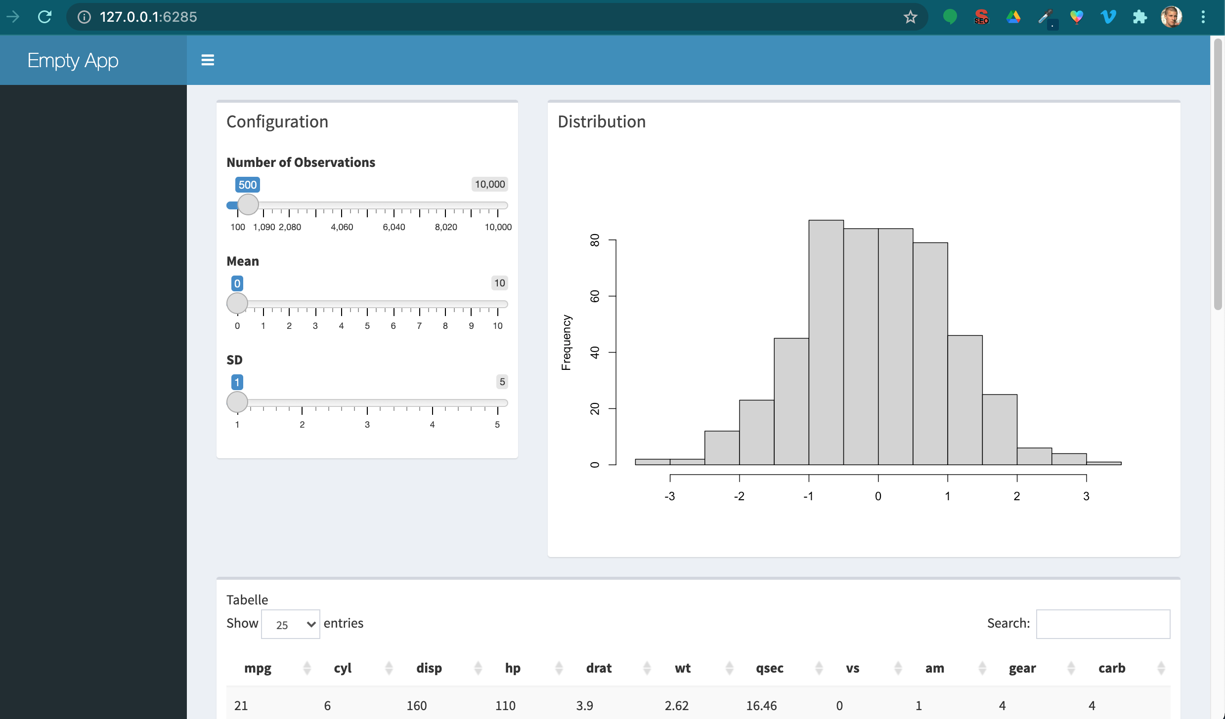
Let’s consider the following web frontend put together with a few lines of R code. Consider the following, simple web fronted that lives in a dedicated user interface R file, called ui.R:
library(shiny)
library(shinydashboard)

dashboardPage(
  dashboardHeader(title = "Empty App"),
  dashboardSidebar(),
  dashboardBody(
    fluidPage(
      fluidRow(
        box(title = "Configuration",
            sliderInput("nobs",
                        "Number of Observations",
                        min = 100,
                        max = 10000,
                        value = 500),
            sliderInput("mean_in","Mean",
                        min = 0,
                        max = 10,
                        value = 0),
            sliderInput("sd_in","SD",
                        min = 1,
                        max = 5,
                        value = 1),
            width = 4),
        box(title = "Distribution",
            plotOutput("dist"),
            width = 8)
      ),
      fluidRow(
        box("Tabelle",
            dataTableOutput("tab"),
            width=12
            )
      )
    )

  )
)
Besides the shiny package itself, the ecosystem around shiny brings popular frontend frameworks from the world outside data science to R. In the above case, a boilerplate library for dashboards is made available through the add-on package {shinydashboard}.
Take a moment to consider what we get readily available at our finger tips: Pleasant user experience (UX) comes from many things. Fonts, readability, the ability to adapt to different screens and devices (responsiveness), a clean, intuitive design and many other aspects. {shinydashboard} adds components like fluidPages or fluidRow to implement a responsive (google me), grid based design using R. Note also how similar the hierarchical, nested structure of the above code is to HTML tagging. (Here’s some unrelated minimal HTML)
<!-- < > denotes an opening, </ > denotes an end tag. -->
<html>
  <body>
  <!-- anything in between tags is affected by the tags formatting.
       In this case bold -->
    <b> some bold title </b>
    <p>some text</p>
  </body>
</html>
{shiny} ships with many widgets6 such as input sliders or table outputs that can simply be placed somewhere on your site. Again, add-on packages provide more widgets and components beyond those that ship with shiny.
6.6.2 Backend
While the frontend is mostly busy looking good, the backend has to do all the hard work, the computing, the querying – whatever is processed in the background based on user input.

Under-the-hood-work that is traditionally implemented in languages like Java, Python or PHP7 can now be done in R. This is not only convenient for the R developer who does not need to learn Java, it’s also incredibly comfy if you got data work to do. Or put differently: who would like to implement logistic regression, random forests or principal component analysis in PHP?
Consider the following minimal backend server.R file which corresponds to the above ui.R frontend file. The anonymous (nameless) function which is passed on to the ShinyServer function takes two named lists, input and output, as arguments. The named elements of the input list correspond to the widgetId parameter of the UI element. In the below example, our well known base R function rnorm takes nobs from the input as its n sample size argument. Mean and standard deviation are set in the same fashion using the user interface (UI) inputs.
library(shiny)

shinyServer(function(input,output){

  output$dist <- renderPlot({
    hist(
      rnorm(input$nobs,
            mean = input$mean_in,
            sd = input$sd_in),
      main = "",
      xlab = ""
      )
  })

  output$tab <- renderDataTable({
    mtcars
  })


})
The vector that is returned from rnorm is passed on to the base R hist which returns a histogram plot. This plot is then rendered and stored into an element of the output list. The dist name is arbitrary but again matched to the UI. The plotOutput function of ui.R puts the rendered plot onto the canvas so it’s on display in people’s browsers. renderDataTable does so in analog fashion to render and display the data table.
6.6.3 Put Things Together and Run Your App
The basic app shown above consists of a ui.R and a server.R file living in the same folder. The most straight forward way to run such an app is to call the runApp() function and provide the location of the folder that contains both of the aforementioned files.
library(shiny)
runApp("folder/that/holds/ui_n_server")
This will use your machine’s built-in web server and run shiny locally on your notebook or desktop computer. Even if you never put your app on a web server and run a website with it this is already a legitimate way to distribute your app. If it was part of an R package, everyone who download your package could use it locally, maybe as a visual inspection tool or way to derive inputs interactively and feed them into your R calculation.
6.6.4 Serve your App
Truth be told, the full hype and excitement of a shiny app only comes into play when you publish your app and make it available to anyone with a browser, not just the R people. Though hosting is a challenge in itself let me provide you a quick shiny specific discussion here. The most popular options to host a shiny app are
software-as-a-service (SaaS). No maintenance, hassle free, but least bang-for-buck. The fastest way to hit the ground running is R Studio’s service shinyapps.io.
on premise aka in house. Either download the open source version of shiny server, the alternative shiny proxy or the R Studio Connect premium solution and install them on your own Virtual machine.
use a shiny server docker image and run a container in your preferred environment.
6.6.5 Shiny Resources
One of the cool things of learning shiny is how shiny and its ecosystem allow you to learn quickly. Here are some of my favorite resources to hone your shiny skills.
online widget galleries like R Studio’s shiny widget gallery that help to ‘shop’ for the right widgets.↩︎
Yup, there is node and javascript on web servers, too, but let’s keep things simple and label javascript clientside here. And yes, shiny server used to require node itself, too.↩︎